Abaqus basic information

hi Abaqus students.

In this post, I will share with you the basic things I know about Abaqus software.

1. First level unit consistency and conversions

Mass	Length	Time	Force	Stress	Energy	Density	Young's Modulus	Gravity
Kg	m	s	N	Pa	J	7.83e+03	2.07e+11	9.806
Kg	cm	s	1.0e-02N			7.83e-03	2.07e+09	9.806e+02
Kg	cm	ms	1.0e+04N			7.83e-03	2.07e+03	9.806e-04
Kg	cm	us	1.0e+10N			7.83e-03	2.07e-03	9.806e-10
Kg	mm	ms	kN	GPa	kN-mm	7.83e-06	2.07e+02	9.806e-03
g	cm	s	dyne	dyne/cm^2	erg	7.83e+00	2.07e+12	9.806e+02
g	cm	us	1.0e+07N	Mbar	1.0e+07Ncm	7.83e+00	2.07e+00	9.806e-10
g	mm	s	1.0e-06N	pa		7.83e-03	2.07e+11	9.806e+03
g	mm	ms	N	MPa	N-mm	7.83e-03	2.07e+05	9.806e-03
ton	mm	s	N	MPa	N-mm	7.83e-09	2.07e+05	9.806e+03
ibf-s^2/in	in	s	ibf	psi	ibf-in	7.33e-04	3.00e+07	386
slug	ft	s	ibf	psf	ibf-ft	1.52e+01	4.32e+09	32.17
kgf-s^2/mm	mm	s	kgf	kgf/mm^2	kgf-mm	7.98e-10	2.11e+04	9.806e+03
Kg	mm	s	mN	1.0e+03pa		7.83e-06	2.07e+08	9.806e+03
g	cm	ms	1.0e+1N	1.0e+05pa		7.83e+00	2.07e+06	9.806e-04

In this case, you need to check the consistency of material properties units, design dimension units, etc. For example, if you have dimension units in millimeters all material properties units must be related to millimeters. For example, if dimension units are used in meters, their density should be in kg / m3 and other related properties should be used. Use the table above for more details. The letter e in that table indicates the Multiplication of ten (10 ×). You can refer to this as e in Abaqus software.

Sometimes we have to transfer the data we have from one unit to another unit, The tables below may be helpful in such situations.

Units:N,m,Kg,S	Units:N,mm,Tonne,S
Length:m	Length:mm
Mass:Kg	Mass:Tonne(T)
Time:Second	Time:Second
Force:Newton	Force:Newton
Energy/Work:Joule(J)	Energy/Work:millijoule(mJ)
Power:Watt(=W=Js)	Power:milliwatt(=mW=mJs)
Density:kg/m^3	Density:T/mm^3
Modulus/Stress:N/m2(=Pa)	Modulus/Stress:N/mm2(=MPa)
Temperature:Kelvin(for temperature differentials,1K=1degree C)	Temperature:Kelvin(for temperature differentials,1K=1degree C)
Conductivity:W/m.C(=J/s/m.C)	Conductivity:mW/mm.C(=mJ/s/mm.C)
Specific Heat:J/Kg.C	Specific Heat:mJ/Tonne.C
Thermal expansion Coefficient:m/m.C(1/C)	Thermal expansion Coefficient:mm/mm.C(1/C)
Flux:W/m2(=J/s/m2)	Flux:mW/mm2(=mJ/s/mm2)
Convection:W/m2.C(=J/s/m2.C)	Convection:mW/mm2.C(=mJ/s/mm2.C)

(Exp.)	Units: N, m, Kg	Units: N, mm, Tonne
Length=50×70mm	Length=0.05×0.07m	Length=50×70mm
Density=4.5g/cm3	Density=4.5e3Kg/m3	Density=4.5e-9Tonne/mm3
Yield Stress=445MPa	Yield Stress=445e6Pa	Yield Stress=445MPa
Elasticity=105GPa	Elasticity=105e9Pa	Elasticity=105e3MPa
Conductivity=16.4W/(m.C)	Conductivity=16.4W/(m.C)	Conductivity=16.4mW/(mm.C)
Specific Heat=523(J/Kg.C)	Specific Heat=523(J/Kg.C)	Specific Heat=523e6(mJ/Tonne.C)
Thermal expansion Coefficient=9.2µm/(m.C)	Thermal expansion Coefficient=9.2e-6m/(m.C)=9.2E-6 (1/C)	Thermal expansion Coefficient=9.2e6mm/(mm.C)=9.2e-6 (1/C)

	Commonly used unit SI-m value	SI-mm value	Mulitification factor from commonly used unit to SI-mm
Stiffness of steel	210GPa(210×10^9Pa)	210000MPa	1000
Density of steel	7850Kg/m^3	7.85×10^-9 tonne/mm^3	10^-12
Gravitational constant	9.81m/s^2	9810mm/s^2	1000
Pressure	1bar(10^5Pa)	0.1MPa	10^-1
Absolute zero temperature	-273.15°C 0 K	°C and K Both are acceptable
Stefan Boltzmann constant	5.67×10^-8 W.m^-2.K^4	5.67×10^-11 mW.mm^-2.K^4	0.001
Universal gas constant	8.31 J.K^-1.mol^-1	8.31×10^3 mJ.K^-1.mol^-1	1000

Second level part creation

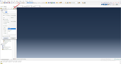
The second level of analysis is to create the required part. In this case, there are different types of part creation methods such as deformable, discrete rigid, analytical rigid, eulerian.

We can select these according to our needs and create a part. For example, you can choose deformable if you plan to perform a brittle or damaged analysis. You can use a discrete rigid or analytical rigid if you want to use a hard, brittle material. Such a rigid part is not subject to any scrutiny. And this does not require any material properties. Using the rigid part will reduce the running time. The rigid part can be used for a hard system like a tool. The eulerian part can be used for a water-like structure.

1mm is 0.001 when given in meters so you can give approximate size as 0.2 when using meter consistent. The approximate size is the size that covers the part dimension. For example, if the length of the object is 150mm, the approximate size may be slightly larger than that, you Can give an approximate size of 200.

Third level material properties creation

In the third stage, the selected and aligned material properties are created. The next step is to create a section and enter the material properties. This material section is then assigned to the part. Thus part became great for its material properties. In this, we can use two or three different properties by dividing the part into two-thirds using a partition.

Fourth level assembly section

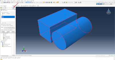
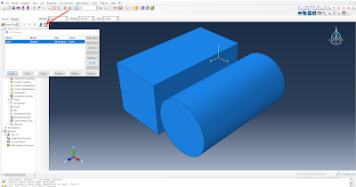
If there is more than one part that you have created, they are assembled in the correct position in the assembly section. In this case, the distance and angle between the two objects can be adjusted.

Fifth level step creation

In this case, the study method required for the study is selected. For example static general, heat transfer, etc.

Sixth level interaction

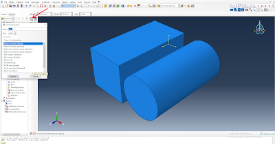
In this case, if two objects touch each other, the required friction force will be given. In this case, we will describe two methods that we need the most. The first method is general contact, in which case any part of an object can interact with any part of another object. Another method is surface to surface contact, in which case only the contact area can be selected. Also in this case the constraint required for rotation like coupling can be given.

Seventh level load boundary conditions

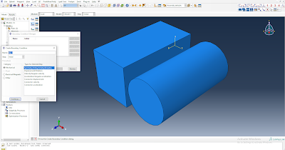
In this case, the required load (ex; pressure, temperature), etc. for the test is given. And the boundary conditions required for the movement of the object are given.

Eighth level mesh

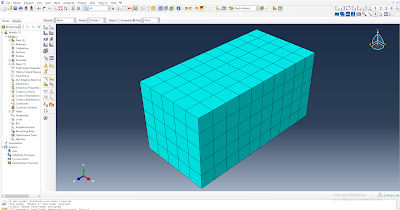
A mesh is like a small atom, which adds material properties to small atoms per part. Use it significantly and you will get results quickly. Used in very small quantities it can cause problems in obtaining accurate results. This method has many variants such as hex, ted, wedge. You can select and use the correct ones.

Ninth level results

After completing the above methods, in this case, go to the job manager and create and continue. After that, we can get the result we want after a short while submit.

Tenth level visualization

The final step is to visualize the results we got and see here.